Heapsort temporal complexity explained

The heapsort algorithm temporal complexity is O(nlgn). In this post, I’ll explain step-by-step why that is the temporal complexity.

We use asymptotic notation to express the running time of an algorithm as a function of the input’s size.

As a short reminder, an algorithm’s (theoretical) temporal complexity is the lowest bound for the function that represents the number of elemental operations (EO) the algorithm must execute to give us a result. In other words, the bound must be asymptotically tight.

So, the steps are as follows:

Find the function that represents the number of elemental operations that the algorithm must execute.
Calculate an asymptotically tight bound.

The theoretical temporal complexity is not dependent on a specific implementation or programming language. So, we will use the pseudo-code for the algorithm to do the analysis.

What is a binary heap?
Heapsort algorithm
Pseudocode for the auxiliary algorithms
MaxHeapify temporal complexity
BuildMaxHeap temporal complexity
Heapsort temporal complexity

What is a binary heap?

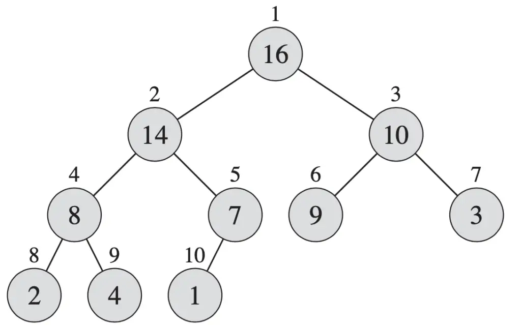
A binary heap is a data structure with the following properties:

All levels of the tree are complete, except probably the lowest level. The lowest level is filled from left to right.
Each node is greater or equal to any of its children.

A consequence of the previous properties is that the height of the tree is h<=lg n, and the root contains the biggest element on the tree.

See the example below.

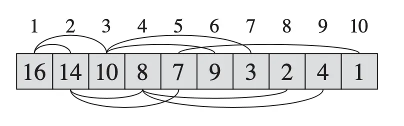
Heap example. Source: Introduction to Algorithms by Cormen.

Even though we represent it as a tree, the actual elements are in an array. In this array, the left child of the element in position i, if exists, is in position 2*i; the right child, if exists, is in position 2*i + 1; and the parent of node i is in position ⎣i/2⎦. In this case, we assume the array starts with the index 1.

See the representation in the array below.

Array representation of a heap. Source: Introduction to Algorithms by Cormen.

Heapsort algorithm

See below the Heapsort algorithm.

Heapsort(A)
    BuildMaxHeap(A)
    For i=A.length Downto 2
            Swap A[1] with A[i]
            A.heapsize = A.heapsize -1
            MaxHeapify(A,1)

As you can see, this algorithm uses two auxiliary algorithms, BuildMaxHeap and Maxheapify. The pseudocode for those other two algorithms is below.

Pseudocode for the auxiliary algorithms

BuildMaxHeap(A)
    A.heapsize = A.length
    For i= ⎣A.length/2⎦ Downto 1
         MaxHeapify(A,i)

MaxHeapify(A, i)
   l = Left(i)
   r = Right(i)
   if l<=A.heapsize and A[l]>A[i]
      largest = l
   else
      largest = i
   if r<=A.heapsize and A[r]>A[largest]
       largest = r
   if largest <>i
       Swap A[i] with A[largest]
       Maxheapify(A, largest)

When you calculate the temporal complexity (I’ll omit “theoretical” from now on, you should know I’m referring to the theoretical temporal complexity) of an algorithm, that uses other algorithms, you should start with the “independent one”.

In our case, Heapsort uses BuildMaxHeap and MaxHeapify, BuildMaxheap uses MaxHeapify, and MaxHeapify does not use any other algorithm.

So, we start with MaxHeapify, then continue with BuildMaxHeap, and lastly, we calculate the temporal complexity of Heapsort.

MaxHeapify temporal complexity

This algorithm assumes that the right and left children of element i are heaps, but element i might not hold the property of being greater than the left and right children.

MaxHeapify(A, i)
   l = Left(i)
   r = Right(i)
   if l<=A.heapsize and A[l]>A[i]
      largest = l
   else
      largest = i
   if r<=A.heapsize and A[r]>A[largest]
       largest = r
   if largest <>i
       Swap A[i] with A[largest]
       Maxheapify(A, largest)

All lines of the pseudocode, except the last one, are executed in constant time. Because A is an array, the operations Left and Right are counted as 1 elementary operation (EO). The same goes for conditionals and assignments that only involve primitive data types or accessing a specific element of an array. So all those steps can be bound by 𝚯(1).

It gets a bit more complex in the last line as it is a recursive call.

Because MaxHeapify will move only in one branch of the tree of root i, because the other one is already a heap, the recursive call can happen in the worst case lg n times. Notice that this number is defined by the height of the subtree.

So, the temporal complexity of MaxHeapify will be O(lg n) + 𝚯(1) = O(lg n).

BuildMaxHeap temporal complexity

BuildMaxHeap(A)
    A.heapsize = A.length
    For i= ⎣A.length/2⎦ Downto 1
         MaxHeapify(A,i)

We know that MaxHeapify has a temporal complexity of O(lg n), and we have an assignment in the first line, which is O(1), and a loop which is O(n/2)=O(n).

So, the temporal complexity in this case will be O(1)+ O(n)*O(lg n) = O(n lg n).

But there is a problem here.

As you should remember when we say the temporal complexity of an algorithm is O(n), or any other asymptotic bound, n is the size of the input.

In our case, the call to MaxHeapify is not defined always by n, being n the size of the array A. Notice that MaxHeapify is called with i as a parameter, where i is the root element on the heap that we want to make sure that the tree with root i is also a heap.

As a consequence, the time complexity of each call to MaxHeapify will depend on the height of the element i on the tree. We also know that the height of the heap is lg n.

Therefore, the total time needed to execute the for loop will be as follows:

∑ h/2^h+1 O(h) = O(n ∑ h/2^h)

The first summation is from h=0 to lg n, the second one is from h=0 to infinity. See the explanation below why we can do such a change.

Notice that the summation from 0 to lg n is less than the same summation from 0 to infinity. This is because h/2^h+1 is a positive number. Using that, the next step is to use the well-known fact that the summation from h=1 to infinity, of h/2^h equals 2. This is called the infinite decreasing geometric series.

So, the final temporal complexity for BuildMaxHeap is:

O(n ∑ h/2^h)=O(2n)=O(n).

Now that we have the temporal complexity of the two auxiliary algorithms, we can calculate the temporal complexity of the heapsort algorithm.