Temporal complexity of iterative algorithms

We use the big-O notation to calculate the temporal complexity of algorithms.

In this post, I’ll show how to calculate the temporal complexity of iterative algorithms.

As a reminder, an algorithm is a finite sequence of steps that, when executed in a certain order, solve a problem.

A problem is a pair (E, S) where E is the input and S is the expected output.

Our goal, when calculating the temporal complexity of an algorithm, is to determine how many elementary operations are in an algorithm. Indeed, it is a counting problem.

Elementary operations
Temporal complexity of conditionals
Temporal complexity of loops
- Graphical view of two examples of temporal complexity
Logarithmic temporal complexity example
Polinomial temporal complexity example

Elementary operations

By elementary operations we mean operations that have a constant execution time, some of them are:

Arithmetic operations
Comparisons (<,>,==)
Conditional statements
Assign a value to a variable
Access to an element in an array or matrix
Return statements
Etc.

After we have a function that represents the number of elementary operations in an algorithm, we can then state that the temporal complexity of that algorithm is the lowest big-O of the number of elementary operations.

For instance, suppose that an algorithm must execute T(n)=4n+5 elementary operations to give a result.

From the big-O notation post, you know that 4n is O(4n+5). However, we cannot say that the temporal complexity of that algorithm is 4n because 4n is not the lowest function that is O(4n+5). The lowest one is n, which is O(4n+5) and also O(4n).

We can now conclude that the temporal complexity of the algorithm that must execute T(n)=4n+5 elementary operations to give us a result, is O(n).

Temporal complexity of conditionals

Let’s see the following example.

double divide(a, b){
        if (b==0){
            throw new Exception("Division by 0 not defined");
        }
        else { 
           result = a/b;
           return result;
       }
  }

The previous example is an algorithm that returns the division of two numbers. It is only for instructional purposes, notice that the use of the variable result is unnecessary.

First, let’s assign the number of elementary operations (EO) at the right of each instruction.

double divide(a, b){
        if (b==0){                                                                           EO=1
            throw new Exception("Division by 0 not defined");  EO=1
        }
        else { 
           result = a/b;                                                                     EO=1
           return result;                                                                   EO=1
       }
  }

Following the sum rule:

Sum rule: if f1 is O(g(x)) and f2 is O(h(x)) ⇒ (f1 +f2)(x) is O(max(|g(x)|,|h(x)|))

We get that T(N) = 1 +1 = 2 in the worst-case scenario.

Now, we use the big-O notation to state that 2 is O(1). This means that f(x)=2 grows more slowly than a certain multiple than g(x)=1.

So, the final answer will be that the temporal complexity of the previous algorithm is O(1).

Temporal complexity of loops

The reasoning for the algorithm above is the same for all iterative algorithms. Let’s see another example where we use loops.

boolean isPrime(n):
    square_root = int(n^0.5) + 1
    for i in range(2, square_root):
        if n % i == 0:
            return False
    return True

Now, a trick for practical use.

square_root = int(n**0.5) + 1

In the line of code above, we are supposed to calculate how many elementary operations must be executed. We have an exponentiation, an addition, and an assignment. There are 3 elementary operations.

However, we know now, that if the number of elementary operations is 5, 10, or 1000000, in all cases, they are O(1). So, from a practical point of view, we don’t count the number of operations, we just state that specific line of code is O(1). It is important to only do it like that when the number of operations does not depend on the size of the input (n in this case).

Let’s go to the for loop.

How many times the for loop is repeated? The square root of n, minus 1.

How many EO are inside the loop? There are three in the worst case. There is a mod operation, a comparison operation, and a return operation.

Now, to calculate the temporal complexity of the loop, we use the product rule:

Product rule: if f1 is O(g(x)) and f2 is O(h(x)) ⇒ (f1 * f2)(x) is O( g(x) * h(x) )

So, in this case, the function that determines the number of EO is T(n)=(√n-1)x3.

Now, we apply the sum rule to add the first 3 EO to the ones of the loop.

The number of EO for the whole algorithm is T(n)=3+3(√n-1).

3 is O(1) and 3(√n-1) is O(√n)

Therefore, we can state that the temporal complexity is O(√n).

A practical way to do this is as follows:

boolean is_prime(n):
    square_root = int(n^0.5) + 1.    O(1)
    for i in range(2, square_root):   O(√n) 
        if n % i == 0:                            O(1)   
            return False                          O(1)
    return True

Therefore, O(√n).

Graphical view of two examples of temporal complexity

Let’s examine, using the definition of big-O, why any constant is O(1) and why 3(√n-1) is O(√n).

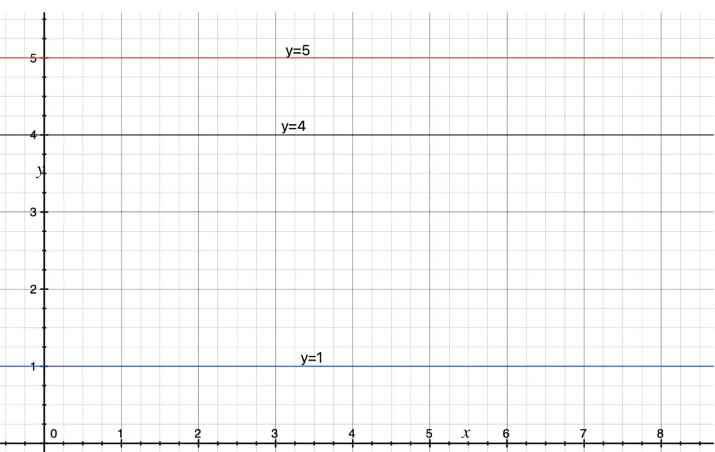
4 is O(1) because there exist C=5 and k=0 such that C*1>=4 for all k>0.

Similarly, for any constant p, we can find C=p+1 such that C*p>=p for all k>0.

So, in practice, anytime you find a sequence of steps that can be executed in constant time, we state that the temporal complexity of that block is O(1).

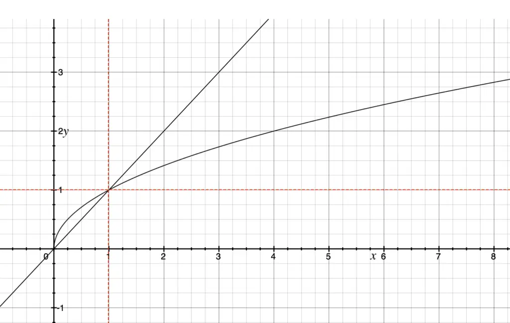
For a similar reason, if you have a number of elementary operations defined by pn, where p is a constant, the temporal complexity is O(n).

Other examples:

T(n)=5n² + 3n + 5 is O(n²), by the sum rule.
T(n)=3n + 4 is O(n), by the sum rule.
T(n)=3n * 4n is O(n²), by the product rule.

Logarithmic temporal complexity example

Something interesting, and usually confusing for students, happens when the variable of a loop doesn’t increase by 1.

Let’s see an example.

print_doubles(n):
    for (int i=1; i<n; i=i*2)
        print (i)

How many times the loop will be executed?

Most will say n/2, and the answer is wrong.

Let’s calculate stating the values that i takes in several cases:

For n = 4:

i=1=2⁰
i=2=2¹

For n=5

i=1=2⁰
i=2=2¹
i=4=2²

For n=6

i=1=2⁰
i=2=2¹
i=4=2²

For n=9

i=1=2⁰
i=2=2¹
i=4=2²
i=8=2³

So, with any iteration, i is a power of 2, and the exponent tells us the number of iterations.

So, the following formula applies.

n=2^p+k, where p is the number of iterations and k is a constant.

To calculate p, we use the following: n=2^p if and only if p=log(n). This is one of the properties of the logarithmic function.

n=2^p+k

n-k=2^p

It follows that p = log(n-k)

Now, we can use big-O notation to state the temporal complexity.

log(n-k) is O(log(n)).

With this, you should easily see that you always need to be aware of the values that the control loop variable takes.

It is generally wrong to just answer O(n) because is a loop. You need to check how many times the loop will be executed.

Polinomial temporal complexity example

Here is another example:

methodX(n):
    for (int i=1; i<n*n; i=i+1)
        print (i)

How many times the loop will be executed?

In this case, it will be repeated until i is equal to or greater than n*n=n². Because i increases in 1 at each repetition, the total number of times the loop will be executed is n².

Therefore, in this case, the temporal complexity is O(n²).

We refer to n as the size of the input. There are common cases as follows:

When the input is an array, the size of the input is usually the size of the array.
When the input is a matrix, the size of the input is the dimension of the matrix, usually nxm.
When the input is a number (as a parameter, like the last example in this post), and the number of OE is a function of that number, then the size of the input is n.
In other cases, we must use common sense.

Next, I’ll show how to calculate the complexity of recursive algorithms.

Table of Contents